Ground-state logic and minimal models

After my undergraduate studies, I joined D-Wave. There, Geordie Rose posed the problem of finding the minimal interaction model capable of universal ground-state quantum computation. The company was already developing hardware based on the transverse-field Ising model. Barahona’s results had established the computational hardness of finding ground states for important classes of classical Ising spin glasses. [48]

The optimization idea behind simulated and physical annealing acquired a quantum formulation through quantum annealing and adiabatic quantum computation. Kadowaki and Nishimori studied quantum annealing in the transverse Ising model. Farhi, Goldstone, Gutmann, and Sipser then formulated an adiabatic computational model that interpolates from an initial Hamiltonian to a final problem Hamiltonian whose ground state encodes a solution. For Boolean problems, that final Hamiltonian is diagonal and can be written in Ising variables, making the problem specification the programmable part of the model. Childs, Farhi, and Preskill then analyzed conditions under which adiabatic computation remains robust to specified control errors and decoherence. Together, these results made the programmable Ising endpoint a concrete structural target: what Boolean logic can its ground space express, and what smallest extension carries the model to universal ground-state quantum computation? [3234]

I studied its low-energy structure by writing Boolean relations as commuting, nonnegative penalty Hamiltonians. A gate is represented by a penalty whose zero-energy space contains precisely its truth-table assignments.

Two input spins enter an AND gate whose output is a third spin; the circuit maps to a three-spin Ising network with pairwise couplings.

The Boolean circuit becomes a three-spin Ising model: the two input wires and the output wire become spins joined by pairwise couplings. [13, 14]

Ground-state spans are logical vector spaces. A single ground space may contain several mutually exclusive classical solutions as basis vectors. Because the constraint algebra is commuting, these propositions remain within one classical context; the construction does not invoke a quantum measurement problem.

Logical gates compose by sharing spins and adding their penalties. A one-body penalty can fix any chosen output value; minimizing the sum then leaves the corresponding satisfying assignments in the ground space. Ancillary spins give exact nonperturbative reductions from commuting many-body constraints to two-body Ising interactions. [13, 14, 21]

The quantum side required noncommuting interactions. Adding controllable XX couplings to the transverse-field Ising resources {ZZ, Z, X} was the smallest extension we found. With Peter Love, I used Feynman–Kitaev history states to prove QMA-completeness for two restricted 2-local Hamiltonian families with one-local X/Z terms and two-local XX/ZZ or ZX/XZ couplings. Perturbative gadgets relate these interaction types. The price of universality is a clock and a history state rather than a single static output configuration. [1, 15]

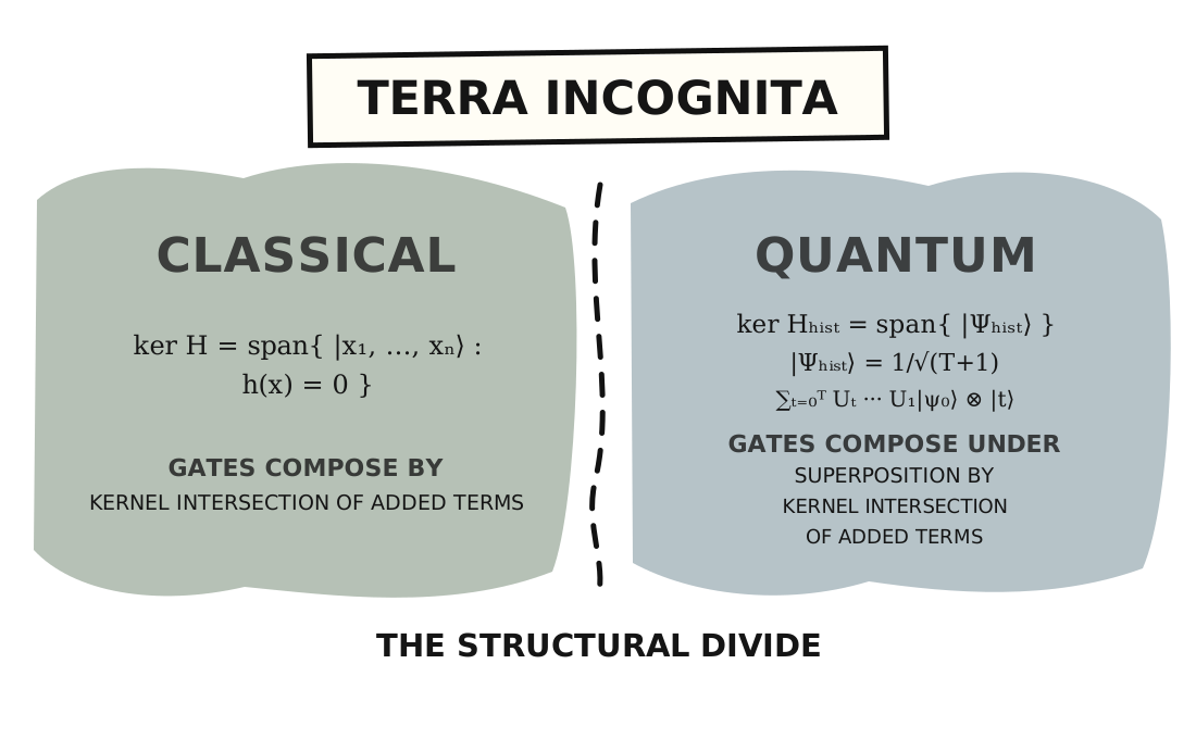
A reconstructed 2007 map of the quantum–classical terra incognita. A classical ground-space kernel and a quantum history-state kernel lie on opposite sides of a dashed boundary labelled the structural divide.

The structural divide · 2007

Classical composition. Gates compose by intersecting the kernels of added terms, producing a Boolean logic of propositions.

Quantum composition. Gates compose under superposition by intersecting the kernels of added terms; at the time, the structure of that logic was less clear.

I searched for a better understanding of how to bridge the quantum–classical terra incognita.

Learn more: Disambiguating “ZX Hamiltonians” Pauli products, interaction families, basis changes, and related spin models

The ZX Hamiltonian vocabulary changed as the result moved among Hamiltonian complexity, verification, annealing, simulation, and experimental work. The term “ZX Hamiltonian” is also used for Hamiltonians built from any two terms in this interaction family.

Here, ZX is Pauli-interaction notation. The product ZpXq applies Pauli Z to qubit p and Pauli X to qubit q. The label HZX names an entire Hamiltonian family containing local X and Z fields and both orientations of the cross-axis coupling, ZX and XZ. “ZX/XZ interaction family” is therefore the more explicit name. [1]

HZZ/XX = ∑p(hpZp + ΔpXp) + ∑p<q(JpqZpZq + KpqXpXq)
HZX/XZ = ∑p(hpZp + ΔpXp) + ∑p<q(JpqZpXq + KpqXpZq)
Name Meaning here Connection to physics
ZX One two-qubit Pauli product, ZX. An effective ZX term is also the entangling component associated with cross-resonance control of superconducting qubits. That later hardware usage names a particular driven interaction, not the full static family above. [53]
HZX The paper’s shorthand for local X,Z fields together with both ZX and XZ couplings. On this page it is written HZX/XZ to expose the complete interaction menu. A mixed-axis, or cross-axis, spin Hamiltonian. The two orientations matter because the couplings can be independently weighted and attached to different ordered endpoints.
HZZ/XX Local X,Z fields together with same-axis ZZ and XX couplings. It contains the transverse-field Ising model when the XX couplings and longitudinal Z fields are removed. More generally, it is an inhomogeneous anisotropic XYZ spin Hamiltonian with its YY coupling set to zero.

A local Hadamard change of basis exchanges X and Z. On one endpoint of a coupling it gives

(𝟙 ⊗ H)(ZZ)(𝟙 ⊗ H) = ZX
(𝟙 ⊗ H)(XX)(𝟙 ⊗ H) = XZ.

Basis relation. On a bipartite interaction graph, applying Hadamard to one sublattice directly exchanges the ZZ/XX and ZX/XZ menus. This explains why the two families are closely related without making their native couplings identical.

Complexity result. The perturbative construction generates the closed real two-body menu {XX, ZZ, ZX, XZ} from either physical pair, together with local X and Z fields. That is the sense in which both restricted families support the universal real history-state construction. [1]

Learn more: Composing Boolean gates by adding commuting Ising penalties The AND construction, penalty functions, Dirac embeddings, graphical maps, and kernels

For the bit set 𝔹 = {0,1}, each row gives a nonnegative penalty, its matrix embedding, graphical form, and allowed zero-energy space. Sharing spins and adding these penalties composes the corresponding Boolean constraints. [13, 14]

An AND constraint and a fixed output
h(x,y,z) = xy − 2xz − 2yz + 3z ≥ 0

The first two bits are the inputs and the third records their AND. The standard vector-space embedding identifies each bit string u with a computational-basis vector |u⟩ and extends the pseudo-Boolean function linearly as a diagonal operator:

Hh = ∑u∈𝔹n h(u) |u⟩⟨u|,   ker Hh = span{ |u⟩ : h(u) = 0 }
H = ∑x,y,z∈𝔹 h(x,y,z) |xyz⟩⟨xyz| = diag(0, 3, 0, 1, 0, 1, 1, 0)
ker H = span{ |000⟩, |010⟩, |100⟩, |111⟩ }
H1(z) = 𝟙xy ⊗ |1⟩⟨1|z,   H∧,z=0 = H + H1(z)
ker H∧,z=0 = span{ |000⟩, |010⟩, |100⟩ } ≅ span{ |00⟩, |01⟩, |10⟩ }

The diagonal entries are ordered by 000, 001, …, 111. The kernel is therefore the complete truth table of AND. Adding H1(z) assigns positive energy whenever the output bit is one, lifting |111⟩. Minimizing the sum fixes z = 0; dropping that fixed output bit gives the isomorphic span of the three allowed input strings. More generally, the zero-energy space of a sum of nonnegative penalties is the intersection of their kernels. [13, 14]

Generator Penalty function Dirac embedding Graphical map Kernel
Penalize 0 h0(x) = 1 − x H0 = |0⟩⟨0| span{|1⟩}
Penalize 1 h1(x) = x H1 = |1⟩⟨1| span{|0⟩}
Equality / wire h=(x,y) = (xy
= xy
H= = |01⟩⟨01| + |10⟩⟨10| span{|00⟩, |11⟩}
NOT hNOT(x,y) = 1 − (xy
= 1 − (xy)
HNOT = |00⟩⟨00| + |11⟩⟨11| span{|01⟩, |10⟩}
COPY hCOPY(x,y,z)
= (xy)² + (xz
HCOPY = ∑x,y,z∈𝔹
hCOPY(x,y,z) |xyz⟩⟨xyz|
span{|000⟩, |111⟩}
AND h(x,y,z)
= xy − 2xz − 2yz + 3z
H = ∑x,y,z∈𝔹
h(x,y,z) |xyz⟩⟨xyz|
span{|000⟩, |010⟩,
|100⟩, |111⟩}

Penalty and Ising conventions. Zero energy marks an allowed assignment: h0(0) = 1 and h0(1) = 0, so h0 penalizes zero; h1 does the reverse. The single triangles depict these unary tensors, while their Dirac embeddings are the diagonal projectors shown alongside them. For binary bits, (xy)² = xy is the equality penalty; for Ising spins it is (1 − sxsy)/2. NOT uses the complementary penalty. COPY and AND are embedded diagonally and extended linearly over the computational basis.

Classical universality. AND and NOT generate every Boolean function; COPY makes reuse of a bit explicit, while equality joins wires. These are computational-basis constraints—COPY does not clone an arbitrary quantum state.

Learn more: Gate composition in the history state by adding non-commuting terms Propagation Hamiltonians, coherent clock states, and the Feynman–Kitaev kernel

Feynman’s Hamiltonian computer supplied the starting point, and Kitaev’s treatment formalized the circuit-to-Hamiltonian history-state construction. It became a basic tool of Hamiltonian complexity: Kempe, Kitaev, and Regev used perturbation theory in establishing the complexity of the 2-local Hamiltonian problem, while Aharonov and collaborators used the construction to prove the polynomial equivalence of adiabatic and circuit quantum computation. [4952]

For a circuit UT ··· U2 U1 acting on a fixed input |ψ0⟩, the state after step t contains the ordered composition Ut ··· U1. The history state pairs every partial computation with a clock value and adds them coherently. The composition law therefore acts through the superposition:

t⟩ = Ut Ut−1 ··· U10
hist⟩ = 1/√(T+1) ∑t=0Tt⟩ ⊗ |t
ker Hhist = span{ |Ψhist⟩ }

Addition again implements composition. Each term imposes one local gate relation. Adding the terms intersects those constraints, so the ordered products Ut ··· U1 appear throughout the single ground state.

The composition now lies under a superposition. The off-diagonal Ut and Ut terms coherently couple successive clock values. Instead of retaining separate satisfying bit strings, the kernel contains a superposition of the entire computational history.

Classical and quantum tensor-network families

On 1 June 2007, while on an extended visit to Alán Aspuru-Guzik’s group at Harvard, I presented in the Oxford Computing Laboratory seminar series work that later appeared in the papers on Boolean problem embeddings into Ising ground spaces and restricted Hamiltonian families for universal adiabatic quantum computation. [1, 13, 45] I began doctoral study at Oxford that October, advised by Samson Abramsky and Bob Coecke. During the doctorate, I extended the earlier ground-state construction into tensor networks, moving from spans of Boolean configurations to individual tensor states formed as superpositions.

The common structure was circuit composition, not a common logic. Tensor networks supplied a language in which Boolean gates, quantum maps, and state preparation could all be represented without identifying their semantics. They also had an established history through Penrose’s graphical tensor calculus, density-matrix renormalization, matrix-product states, and projected entangled-pair states. The work described here developed algebraic, computational, categorical, and open-system questions within those traditions. [28, 3538]

Conceptually, this was the same compositional structure with two changes. First, the graphical notation now came from quantum circuits. Cutting a CNOT diagram across its internal connection exposes XOR and COPY tensors: complementary structures that came to be drawn as two-colored spiders. [16, 46] Second, the Hamiltonian construction could assign several positive energies to rejected bit strings because taking the kernel discarded every nonzero level. The corresponding relational tensor instead required Boolean coefficients: zero for a rejected assignment and one for an accepted assignment.

Learn more: The AND/COPY/scalar calculus Boolean support functions, quantum-state superpositions, and tensor contraction
Two matching diagrams. Reading an AND tensor from its output toward its inputs and postselecting the output to one produces the state ket eleven; postselecting the output to zero produces ket zero zero plus ket zero one plus ket one zero.
Postselection turns the AND gate into a quantum state. Reading the tensor from its output toward its inputs, postselecting its output to ⟨0| produces |00⟩ + |01⟩ + |10⟩; postselecting to ⟨1| produces |11⟩. Redrawn from Figure 5 of Categorical Tensor Network States under CC BY 3.0. [BCJ11]

The conversion flattens a nonnegative penalty h to its Boolean support function fh(u) = 𝟙[h(u) = 0]. It is one on the allowed assignments and zero on the rejected ones, and becomes the tensor coefficient directly. For the AND relation, the same four satisfying assignments that formed a ground-space basis now form one unnormalized superposition:

|Tf⟩ = ∑u∈𝔹n f(u) |u
ker H = span{ |000⟩, |010⟩, |100⟩, |111⟩ }
|AND⟩ = |000⟩ + |010⟩ + |100⟩ + |111⟩.
Tensor Boolean support function Resulting quantum state
Fix 0 f0(x) = 𝟙[x = 0] |0⟩
Fix 1 f1(x) = 𝟙[x = 1] |1⟩
Wire f=(x,y) = 𝟙[x = y] |00⟩ + |11⟩
COPY fCOPY(x,y,z) = 𝟙[x = y = z] |000⟩ + |111⟩
XOR fXOR(x,y,z) = 𝟙[z = xy] |000⟩ + |011⟩ + |101⟩ + |110⟩
AND f(x,y,z) = 𝟙[z = xy] |000⟩ + |010⟩ + |100⟩ + |111⟩

Locality was decisive for the Hamiltonian construction because physical interaction terms had to be reduced to two-body form. It was less restrictive for tensor networks, where higher-arity tensors can be used directly. The underlying logical composition nevertheless remained the same: identify shared variables and compose their relations. Hamiltonians implement that rule by adding penalties and intersecting kernels; tensor networks implement it by joining wires and contracting shared indices. [BCJ11]

Learn more: Tensor-network contractions for counting How plus states turn a Boolean tensor network into the number of satisfying assignments

Let f: 𝔹n → 𝔹 be a Boolean formula. Fixing its output to one gives the Boolean quantum state |ψf⟩, whose basis vectors are precisely the inputs for which f is one. Closing every variable wire with the unnormalized plus bra ⟨+| = ⟨0| + ⟨1| assigns weight one to every bit string and adds the accepted terms. The fully contracted network therefore returns the number of satisfying assignments. [BMT15]

Redrawn Figure 1 showing a Boolean function as a triangular tensor with input wires, followed by two copies whose outputs are fixed to one and whose variable wires are contracted.
A Boolean state and its contraction. In the left diagram, the triangle abstracts fSAT with free variable wires. In the right diagram, each output is fixed to one and the resulting Boolean state is contracted with a reflected copy. The closed contraction is its squared norm and therefore counts the satisfying inputs. Redrawn from Figure 1 of Tensor Network Contractions for #SAT. [BMT15]
f⟩ = ∑x∈𝔹n f(x) |x
⟨+|nf⟩ = ∑x∈𝔹n f(x) = #f−1(1)

Worked example. For f(x,y,z) = (xy) ∧ z, the Boolean state is

f⟩ = |011⟩ + |101⟩ + |111⟩
⟨+|⊗3f⟩ = 1 + 1 + 1 = 3.

Because the amplitudes are Boolean, each satisfying assignment contributes exactly one: no rejected assignment contributes, and there are no relative weights to distort the count. Equivalently, the squared norm satisfies ‖ψf‖² = ∑x f(x). Deciding whether this scalar is nonzero recovers satisfiability; evaluating its value is the corresponding counting problem. [BMT15]

Redrawn graphical Cauchy-Schwarz inequality for a tensor network partitioned into two halves x and y.
Cauchy–Schwarz for a partitioned contraction. Cutting a closed network into halves X and Y makes its value an inner product. Two copies of the cross-contraction are bounded by the product of the two self-contractions; equality holds only when the halves are proportional. Redrawn from the graphical inequality in Theorem 29 of Tensor Network Contractions for #SAT. [BMT15]
f ∈ SAT ⇔ #f = ‖ψf‖² > 0
|𝒞{X,Y}|² ≤ 𝒞{X,X} 𝒞{Y,Y}
(#f)² ≤ 𝒞{X,X} 𝒞{Y,Y}
𝒞{X,X} 𝒞{Y,Y} = 0 ⇒ #f = 0

This places a one-sided bound around the decision problem. If either self-contraction on the right vanishes, then the bound forces #f = 0 and the formula is unsatisfiable. A positive upper bound alone does not prove satisfiability; the exact decision remains whether ‖ψf‖ is nonzero. [BMT15]

With Stephen Clark and Dieter Jaksch, I developed the categorical tensor-network-state factorization, including an explicit decomposition of arbitrary states and an AND/COPY/|−⟩ computational-universality construction. [BCJ11]

Model statistics

At the ISI Foundation in Torino from 2012, I worked with collaborators to apply methods from complex networks to quantum systems. The work brought the continuous-time quantum-walk model together with scale-free network growth, the Bianconi–Barabási Bose-statistics mapping for evolving networks, entanglement percolation, and quantum random networks. [3943]

Logic and tensor algebra answered exact structural questions but said less about ensembles and emergent behavior. Network science suggested a different question: what can patterns of connection reveal that isolated components do not?

We connected quantum walks to node degree, formulated community detection through transport and distinguishability, and introduced chiral quantum walks. The chiral effect was later demonstrated experimentally on a three-qubit NMR processor. In the reverse direction, spectral entropies and distances supplied tools for comparing classical networks. [17, 19, 26, 27, 47]

The exchange runs both ways: methods from complex networks describe collective quantum behavior, while quantum information supplies tools for comparing classical networks. These papers form part of the early literature connecting quantum dynamics with complex-network observables. The 2019 review Complex Networks from Classical to Quantum organized these links without claiming a sole origin for the subject. [12]

Limits of parameter space

Network statistics later shaped my return to Hamiltonian optimization and the study of variational quantum algorithms. Variational eigensolvers and QAOA replace a long adiabatic path with tunable circuits and a classical optimization loop, making the geometry and statistics of parameter space part of the computational question.

Random satisfiability ensembles exposed reachability deficits in QAOA: even with usable gradients, a fixed-depth circuit may exclude the target states. Parameter concentration and training saturation revealed additional limits that arise from the model rather than the optimizer. [79]

Conversely, we derived precise universality conditions for a class of one-dimensional QAOA constructions, with extensions to specified graph and hypergraph cost Hamiltonians, and proved feed-forward variational quantum computation universal. Related work linked barren plateaus to locality and abrupt trainability changes to circuit depth. [2, 20, 22, 23]

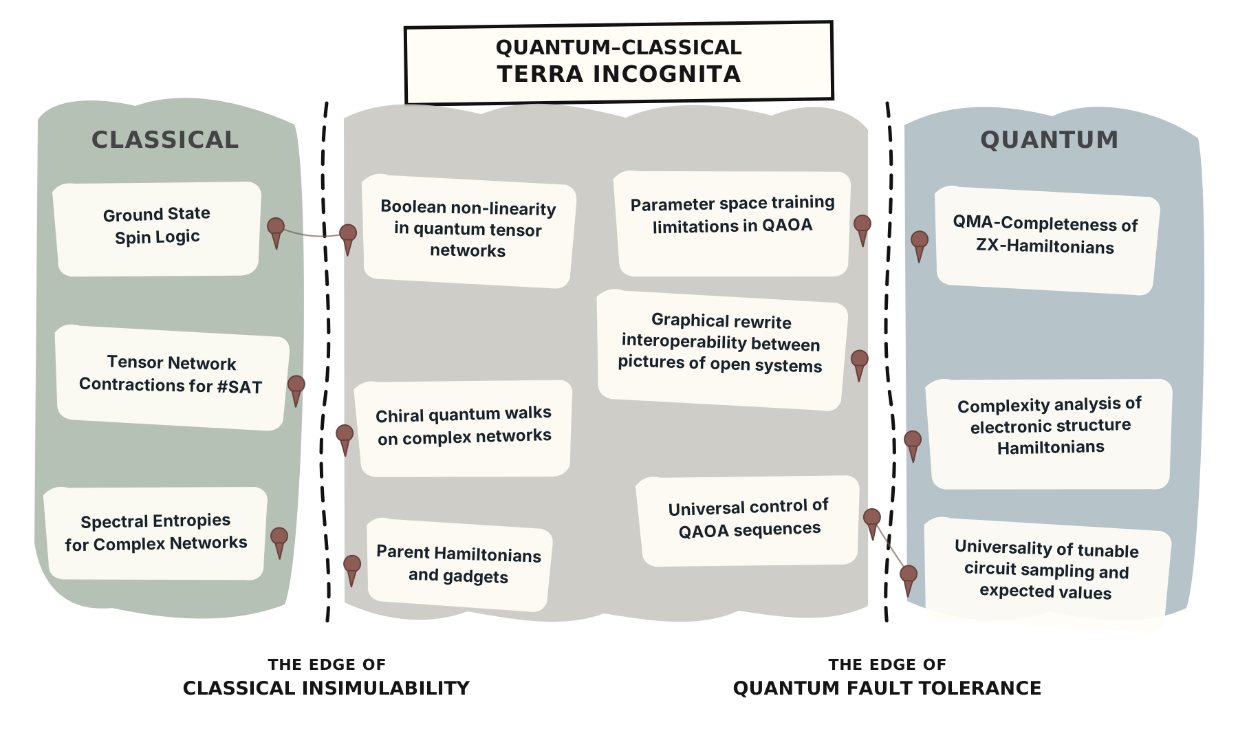
The original divide eventually separated into two limits: classical insimulability and fault-tolerant universal quantum computation. Between them lie structured, restricted, noisy, and trainable models whose computational status remains unresolved.

Selected research topics placed across classical, terra incognita, and quantum regimes divided by the edge of classical insimulability and the edge of quantum fault tolerance.
Conceptual map of the research. The work studies how interactions, composition rules, and model statistics move computational models toward—or away from—the two limiting boundaries.

Within the terra incognita around the edge of classical insimulability: Ground State Spin Logic; Tensor Network Contractions for #SAT; Spectral Entropies for Complex Networks; Boolean non-linearity in quantum tensor networks; Chiral quantum walks on complex networks; Parent Hamiltonians and gadgets.

Around the edge of quantum fault tolerance: Parameter-space training limitations in QAOA; graphical rewrite interoperability between pictures of open systems; precise universality conditions for specified QAOA constructions; QMA-completeness of two restricted 2-local Hamiltonian families; complexity analysis of electronic-structure Hamiltonians; universality of tunable-circuit sampling and expected values.

Research table

The table organizes cited results across Physical Model → Programming Language → Emergent Properties. Read each row from left to right; numbers identify sources below.

Physical Model Programming Language Emergent Properties
Ising Hamiltonians realize spans of Boolean predicates as exact ground spaces, with energy minimization inducing a distributive lattice of physically synthesizable solution spaces [13,14,21]. The algebra of minimization embeds composable logical gates and exactly synthesizes prescribed bit-string ground spaces, providing an algebraic solution to the ground-state inverse Ising problem [13,14,21]. Model statistics reveal QAOA reachability deficits in density-ordered random SAT, showing that limitations can arise from the reachable state space rather than the optimizer. Related work analyzes parameter concentration and layerwise training saturation [7-9].
ZX-Hamiltonian ground-state models are QMA-complete and universal for energy-based models of quantum computation [1]. This work used Hamiltonian complexity as a predictive tool for hardware design by identifying the noncommuting, sign-changing two-body couplers needed to pass from transverse-Ising annealing to universal ground-state quantum computation [1].

Real-valued Feynman-Kitaev history states encode universal quantum computation [1,49,50].

Perturbative gadgets enable ZZ/XX ↔ ZX interoperability [1]; a fourth-order gadget synthesizes YY from ZZ/XX after complete third-order cancellation [15]. Together, these constructions give access to every real Pauli string [1,15].

Access to every real Pauli string brings electronic-structure Hamiltonians within the universal low-energy framework [1,3,15].

Separately, gate-model resource estimates established explicit complexity bounds for molecular-energy calculations [3]. — A Molecular Physics Young Author Prize was awarded to James D. Whitfield for this paper in the 2011 prize cycle; the award was announced in 2012.

Ground-state spin logic [13,14,21], tensor networks, quantum circuits, and graphical calculus [4,6,44] provide the models in this part of the work.

We proved universality results for two different tensor families: AND/COPY/scalar tensor networks are expressively complete, while AND/COPY/|−⟩ tensor networks are quantum computationally universal [4,44].

Graphical rewrites make canonical representations of open quantum systems interoperable, allowing calculations to move systematically between their different mathematical pictures [6].

Tensor algebra, rather than geometry alone, controls contractibility: bialgebra and Hopf rewrites make finite-Abelian lattice-gauge tensor networks exactly contractible, while #SAT instances are polynomial-time tractable when their tensor representations contain O(log n) COPY tensors and have polynomially bounded fan-out [5,24].

Closed tensor diagrams generate complete local-unitary invariants for matrix-product states, including Rényi entropies [25].

A common operator framework links tight-binding transport, stochastic mechanics, and mass-action kinetics, clarifying their shared mathematics and distinct physics [12,18]; quantum degree distributions and community detection turn network structure into state-dependent observables [26,27]. Broken time-reversal symmetry turns loop phases into a control language for directional transport, defining chiral quantum walks [17]. Creation-annihilation and coherent-state mathematics gives new proofs of major reaction-network theorems and identifies Dirichlet forms as a stochastic-quantum boundary [18]. Spectral entropy turns Laplacian diffusion into information-theoretic tools for comparing, clustering, and inferring networks [19]. Together, these five papers form a coherent body of work on complex networks [12,17,19,26,27].

Parameterized-quantum-circuit sampling is computationally universal, elevating variational circuit architectures from heuristic ansätze to a formal model of quantum computation [2]. The work was an APS Editors’ Suggestion and was published as a Letter.

A combinatorial quantum-circuit area law makes hardware connectivity and circuit depth structural limits on low-depth expressibility [2].

A class of one-dimensional QAOA constructions is universal under precise interaction and symmetry conditions, with extensions to specified graph and hypergraph cost Hamiltonians [23].

Gradient-variance bounds identify Pauli-term causal-cone width as a structural control on barren plateaus, linking trainability to cost-function locality and ansatz structure [22].

Learning k-body gates exhibits a sharp depth threshold: one additional layer can switch the circuit from unlearnable to perfectly learnable [20].

Sources and paper links

Parts of this work are synthesized in the reviews Quantum Machine Learning [10], Tensor Networks in a Nutshell [11], and Complex Networks from Classical to Quantum [12].

[1]Realizable Hamiltonians for universal adiabatic quantum computers J. Biamonte and P. Love Physical Review A 78, 012352 (2008). DOI: 10.1103/PhysRevA.78.012352.

[2]Universal variational quantum computation J. Biamonte Physical Review A 103, L030401 (2021). APS Editors’ Suggestion; Letter. DOI: 10.1103/PhysRevA.103.L030401.

[3]Simulation of electronic structure Hamiltonians using quantum computers J. Whitfield, J. Biamonte, and A. Aspuru-Guzik Molecular Physics 109, 735 (2011). DOI: 10.1080/00268976.2011.552441. — A Molecular Physics Young Author Prize was awarded to James D. Whitfield for this paper in the 2011 prize cycle; the award was announced in 2012.

[4]Categorical tensor network states J. Biamonte, S. Clark, and D. Jaksch AIP Advances 1, 042172 (2011). DOI: 10.1063/1.3672009.

[5]Tensor network contractions for #SAT J. Biamonte, J. Morton, and J. Turner Journal of Statistical Physics 160, 1389–1404 (2015). DOI: 10.1007/s10955-015-1276-z.

[6]Tensor networks and graphical calculus for open quantum systems C. J. Wood, J. D. Biamonte, and D. G. Cory Quantum Information & Computation 15, 759–811 (2015). DOI: 10.26421/QIC15.9-10-3.

[7]Reachability deficits in quantum approximate optimization V. Akshay, H. Philathong, M. Morales, and J. Biamonte Physical Review Letters 124, 090504 (2020). DOI: 10.1103/PhysRevLett.124.090504.

[8]Parameter concentrations in quantum approximate optimization V. Akshay, D. Rabinovich, E. Campos, and J. Biamonte Physical Review A 104, L010401 (2021), Letter. DOI: 10.1103/PhysRevA.104.L010401.

[9]Training saturation in layerwise quantum approximate optimisation E. Campos, D. Rabinovich, V. Akshay, and J. Biamonte Physical Review A 104, L030401 (2021), Letter. DOI: 10.1103/PhysRevA.104.L030401.

[10]Quantum machine learning J. Biamonte, P. Wittek, N. Pancotti, P. Rebentrost, N. Wiebe, and S. Lloyd Nature 549, 195–202 (2017). DOI: 10.1038/nature23474.

[11]Tensor Networks in a Nutshell J. Biamonte and V. Bergholm arXiv:1708.00006 (2017). DOI: 10.48550/arXiv.1708.00006.

[12]Complex networks from classical to quantum J. Biamonte, M. Faccin, and M. De Domenico Communications Physics 2, 53 (2019). DOI: 10.1038/s42005-019-0152-6.

[13]Nonperturbative k-body to two-body commuting conversion Hamiltonians and embedding problem instances into Ising spins J. Biamonte Physical Review A 77, 052331 (2008). DOI: 10.1103/PhysRevA.77.052331.

[14]Ground-state spin logic J. Whitfield, M. Faccin, and J. Biamonte Europhysics Letters 99, 57004 (2012). DOI: 10.1209/0295-5075/99/57004.

[15]Hamiltonian gadgets with reduced resource requirements Y. Cao, R. Babbush, J. Biamonte, and S. Kais Physical Review A 91, 012315 (2015). DOI: 10.1103/PhysRevA.91.012315.

[16]Categorical quantum circuits V. Bergholm and J. Biamonte Journal of Physics A: Mathematical and Theoretical 44, 245304 (2011). DOI: 10.1088/1751-8113/44/24/245304.

[17]Quantum transport enhancement by time-reversal symmetry breaking Z. Zimboras, M. Faccin, Z. Kadar, J. Whitfield, B. Lanyon, and J. Biamonte Scientific Reports 3, 2361 (2013). DOI: 10.1038/srep02361.

[18]Quantum Techniques in Stochastic Mechanics J. C. Baez and J. Biamonte World Scientific (2017). DOI: 10.1142/10623.

[19]Spectral entropies as information-theoretic tools for complex network comparison M. De Domenico and J. Biamonte Physical Review X 6, 041062 (2016). DOI: 10.1103/PhysRevX.6.041062.

[20]Abrupt transitions in variational quantum circuit training E. Campos, A. Nasrallah, and J. Biamonte Physical Review A 103, 032607 (2021). DOI: 10.1103/PhysRevA.103.032607.

[21]On the Mathematical Structure of Quantum Models of Computation Based on Hamiltonian Minimisation J. Biamonte Doctor of Science habilitation, Moscow Institute of Physics and Technology (2022). DOI: 10.48550/arXiv.2009.10088.

[22]On barren plateaus and cost function locality in variational quantum algorithms A. V. Uvarov and J. D. Biamonte Journal of Physics A: Mathematical and Theoretical 54, 245301 (2021). DOI: 10.1088/1751-8121/abfac7.

[23]On the universality of the quantum approximate optimization algorithm M. E. S. Morales, J. D. Biamonte, and Z. Zimboras Quantum Information Processing 19, 291 (2020). DOI: 10.1007/s11128-020-02748-9.

[24]Algebraically contractible topological tensor network states S. J. Denny, J. D. Biamonte, D. Jaksch, and S. R. Clark Journal of Physics A: Mathematical and Theoretical 45, 015309 (2012). DOI: 10.1088/1751-8113/45/1/015309.

[25]Tensor network methods for invariant theory J. Biamonte, V. Bergholm, and M. Lanzagorta Journal of Physics A: Mathematical and Theoretical 46, 475301 (2013). DOI: 10.1088/1751-8113/46/47/475301.

[26]Degree distribution in quantum walks on complex networks M. Faccin, T. Johnson, J. Biamonte, S. Kais, and P. Migdał Physical Review X 3, 041007 (2013). DOI: 10.1103/PhysRevX.3.041007.

[27]Community detection in quantum complex networks M. Faccin, P. Migdał, T. H. Johnson, V. Bergholm, and J. D. Biamonte Physical Review X 4, 041012 (2014). DOI: 10.1103/PhysRevX.4.041012.

[28]Applications of negative dimensional tensors R. Penrose Combinatorial Mathematics and Its Applications, 221–244 (1971).

[29]A categorical semantics of quantum protocols S. Abramsky and B. Coecke Proceedings of the 19th Annual IEEE Symposium on Logic in Computer Science (2004). DOI: 10.48550/arXiv.quant-ph/0402130.

[30]A survey of graphical languages for monoidal categories P. Selinger New Structures for Physics, 289–355 (2011). DOI: 10.1007/978-3-642-12821-9_4.

[31]Picturing Quantum Processes B. Coecke and A. Kissinger Cambridge University Press (2017). DOI: 10.1017/9781316219317.

[32]Quantum annealing in the transverse Ising model T. Kadowaki and H. Nishimori Physical Review E 58, 5355–5363 (1998). DOI: 10.1103/PhysRevE.58.5355.

[33]Quantum computation by adiabatic evolution E. Farhi, J. Goldstone, S. Gutmann, and M. Sipser arXiv:quant-ph/0001106 (2000). DOI: 10.48550/arXiv.quant-ph/0001106.

[34]Robustness of adiabatic quantum computation A. M. Childs, E. Farhi, and J. Preskill Physical Review A 65, 012322 (2001). DOI: 10.1103/PhysRevA.65.012322.

[35]Density matrix formulation for quantum renormalization groups S. R. White Physical Review Letters 69, 2863–2866 (1992). DOI: 10.1103/PhysRevLett.69.2863.

[36]Finitely correlated states on quantum spin chains M. Fannes, B. Nachtergaele, and R. F. Werner Communications in Mathematical Physics 144, 443–490 (1992). DOI: 10.1007/BF02099178.

[37]Renormalization algorithms for quantum many-body systems in two and higher dimensions F. Verstraete and J. I. Cirac arXiv:cond-mat/0407066 (2004). DOI: 10.48550/arXiv.cond-mat/0407066.

[38]Matrix product states and projected entangled pair states: Concepts, symmetries, theorems J. I. Cirac, D. Pérez-García, N. Schuch, and F. Verstraete Reviews of Modern Physics 93, 045003 (2021). DOI: 10.1103/RevModPhys.93.045003.

[39]Emergence of scaling in random networks A.-L. Barabási and R. Albert Science 286, 509–512 (1999). DOI: 10.1126/science.286.5439.509.

[40]Bose–Einstein condensation in complex networks G. Bianconi and A.-L. Barabási Physical Review Letters 86, 5632–5635 (2001). DOI: 10.1103/PhysRevLett.86.5632.

[41]Entanglement percolation in quantum networks A. Acín, J. I. Cirac, and M. Lewenstein Nature Physics 3, 256–259 (2007). DOI: 10.1038/nphys549.

[42]Quantum random networks S. Perseguers, M. Lewenstein, A. Acín, and J. I. Cirac Nature Physics 6, 539–543 (2010). DOI: 10.1038/nphys1665.

[43]Quantum computation and decision trees E. Farhi and S. Gutmann Physical Review A 58, 915–928 (1998). DOI: 10.1103/PhysRevA.58.915.

[44]A simple proof that Toffoli and Hadamard are quantum universal D. Aharonov arXiv:quant-ph/0301040 (2003). DOI: 10.48550/arXiv.quant-ph/0301040.

[45]Some Models of Quantum Computation J. Biamonte Oxford Computing Laboratory seminar, 1 June 2007. Oxford Advanced Seminar on Informatic Structures archive.

[46]Interacting quantum observables: Categorical algebra and diagrammatics B. Coecke and R. Duncan New Journal of Physics 13, 043016 (2011). DOI: 10.1088/1367-2630/13/4/043016.

[47]Chiral quantum walks D. Lu, J. D. Biamonte, J. Li, H. Li, T. H. Johnson, V. Bergholm, M. Faccin, Z. Zimborás, R. Laflamme, J. Baugh, and S. Lloyd Physical Review A 93, 042302 (2016). DOI: 10.1103/PhysRevA.93.042302.

[48]On the computational complexity of Ising spin glass models F. Barahona Journal of Physics A: Mathematical and General 15, 3241–3253 (1982). DOI: 10.1088/0305-4470/15/10/028.

[49]Quantum Mechanical Computers R. P. Feynman Optics News 11(2), 11–20 (1985). DOI: 10.1364/ON.11.2.000011.

[50]Classical and Quantum Computation A. Yu. Kitaev, A. H. Shen, and M. N. Vyalyi Graduate Studies in Mathematics 47, American Mathematical Society (2002). DOI: 10.1090/gsm/047.

[51]The Complexity of the Local Hamiltonian Problem J. Kempe, A. Kitaev, and O. Regev SIAM Journal on Computing 35, 1070–1097 (2006). DOI: 10.1137/S0097539704445226.

[52]Adiabatic Quantum Computation Is Equivalent to Standard Quantum Computation D. Aharonov, W. van Dam, J. Kempe, Z. Landau, S. Lloyd, and O. Regev SIAM Journal on Computing 37, 166–194 (2007). DOI: 10.1137/S0097539705447323.

[53]Effective Hamiltonian Models of the Cross-Resonance Gate E. Magesan and J. M. Gambetta Physical Review A 101, 052308 (2020). DOI: 10.1103/PhysRevA.101.052308.