Herve Lombaert

Research Projects Algorithms School Presentations Schedule

Region based segmentation with levelsets

Edge based segmentations are intuitive since edges usually show an object boundary. However in some or many cases, edges are not sharp or are simply not there. Region based segmentations is a solution to this problem. Here is an example using a level set framework.

Edge based segmentation

When trying to isolate an object, its edges are good hints for the object boundary. That is why typical edge based objective functions make use of the gradient $\nabla I$. In a level set framework, high gradients should stop motion, and low gradients should allow the level set motion. For example, motion can be the inverse of the gradient, or it can be its gaussian:

$$\begin{eqnarray*} F & = & \frac{1}{1+\lambda\vert\nabla I\vert}, \textrm{or}\\ F & = & e^{-\frac{\vert\nabla I\vert^2}{2\sigma^2}} \end{eqnarray*}$$

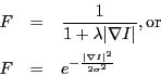
Here, the parameter $\left.\lambda\right.$ or $\left.\sigma\right.$ defines the range of penalizing gradient values: if $\left.\lambda\right.$ is high or if $\left.\sigma\right.$ is low then only the strongest gradients will stop motion.

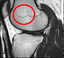
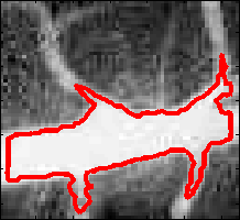
When an object boundary is obvious (see figure below), these objective functions work well.

Figure: Level sets using $F=\left.e^{-\frac{\vert\nabla I\vert^2}{2\sigma^2}}\right.$

(a) Initial contour	(b) Final contour

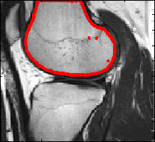
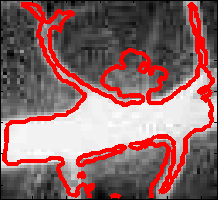
However if the object boundary is not well defined, a weak gradient will not stop the contour. Changing the parameter $\left.\lambda\right.$ or $\left.\sigma\right.$ will possibly slow down the level set motion but it will not prevent the contour to go beyond the boundary. There will be leakage in the neighboring regions as shown in the figure below.

Figure: Level sets using $F=e^{-\frac{\vert\nabla I\vert^2}{2\sigma^2}}$

(a) Initial contour	(b) Intermediate step	(c) Leakage

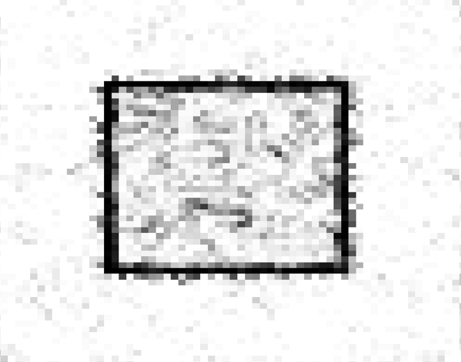
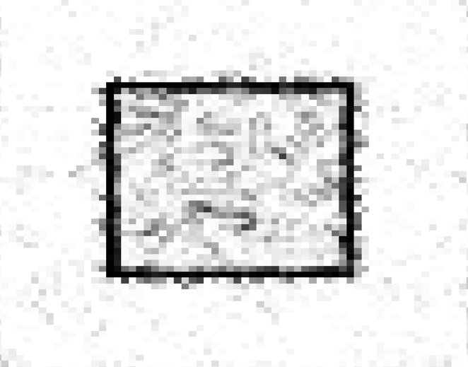
Now, simple synthetic examples will be used in order to illustrate the leakage, and this will help find a solution. The figure below shows an ideal situation with a bright square on a dark background. Its gradient shows a clear boundary. The level set will be stopped there.

Figure: In ideal condition, edge based segmentations work

(a) Ideal solution	(b) Clear gradient	(c) Contour matches

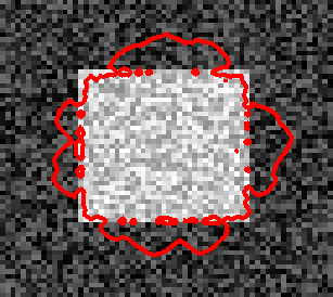
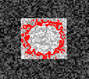
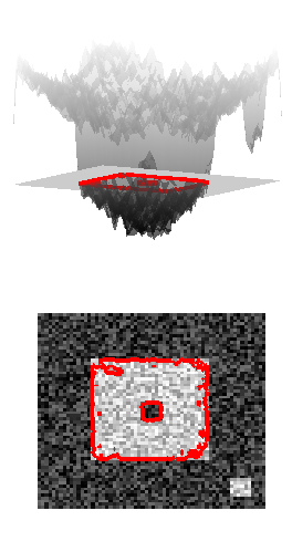
To get closer to real situations, a gaussian noise has been added to the last image. It is still possible to see a bright square on a dark background, but the image gradient does not show a clear single boundary any more. Some spots on the boundary have a weak gradient. This is where leakage will happen as shown in the figure below:

Figure 4: In real conditions, edge based segmentation leaks

(a) Noisy image	(b) Weak gradient	(c) Contour leaks

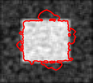
Filtering the image may help, but there is a chance the edges get blurred and leakage will then still occur. In any case, the image is modified and information may be lost. Below is an example of bluring with a gaussian filter, the gradient looks better, but there is still a leakage.

Figure 5: In real conditions, edge based segmentation leaks

(a) Noisy image	(b) Weak gradient	(c) Contour leaks

Region based

The segmentation problem can be tackled differently: instead of looking for boundaries, we look for regions. That means the objective function should enhance regions rather than boundaries. In a level set framework, two regions are easily known with $\left.\phi<0\right.$, inside the contour, and with $\left.\phi>0\right.$, outside the contour. The objective function can measure the homogeneity of both regions.

One way of measuring the homogeneity of a region is with the least squared mean. For this, the mean of pixel intensities of each region is needed:

$$\begin{eqnarray*} \mu_0 & = & \frac{1}{n_0}\sum_{\phi<0} I(i,j)\\ \mu_1 & = & \frac{1}{n_1}\sum_{\phi>0} I(i,j) \end{eqnarray*}$$

with here n₀ the number of pixels inside the contour, n₁ the number of pixels outside the contour. The least squared mean is then:

$$\begin{eqnarray*} F & = & \left.\sum_{\phi<0}\right. \left(I(i,j)-\mu_0\right)^2 + \left.\sum_{\phi>0}\right. \left(I(i,j)-\mu_1\right)^2 \end{eqnarray*}$$

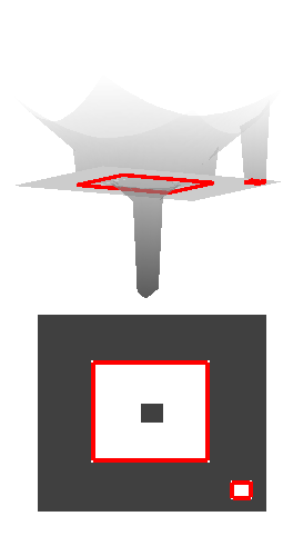
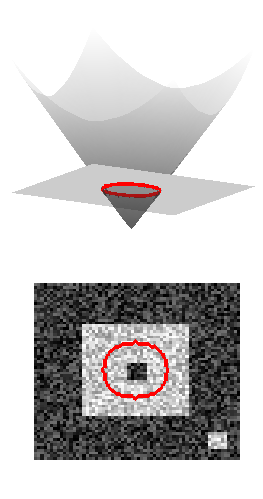
With this objective function, if a pixel has an intensity too different than the mean of region where he is currently classified, it will be penalized. If its intensity is closer to the mean of the other region, the level sets will eventually classify this pixel in the other region. The example below shows how this objective function behaves in the previous problem.

Figure 6: Region based segmentation with the least squared mean

(a) Noisy image	(b) Intermadiatekstep	(c) The homogeneous regions

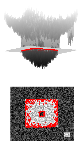
As the level sets evolve, pixels get classified in the region where the mean is closer to the pixel intensity. However, the previous object function is always positive, that means the level sets cannot move back or undo a decision. If a pixel is wrongly classified within an initial contour, it will remain misclassified. This is shown in the figure below.

Figure: Misclassification when $\left.F>0\right.$

(a) Initial contour	(b) Contour only grows outward	(c) Final contour

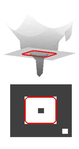
From the previous example, the surface $\left.\phi\right.$ is shown, the force always positive makes the surface only move downward. The contour can then only grow outward. In such a situation, the dark square inside the initial contour cannot be classified as a background. For that to happen, the surface would have to move upward.

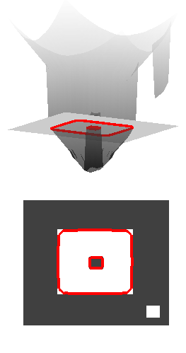
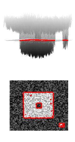
Instead of using the squared mean, the plain difference to the mean would allow negative forces.

$$\begin{eqnarray*} F & = & \left.\sum_{\phi<0}\right. \left(I(i,j)-\mu_0\right) + \left.\sum_{\phi>0}\right. \left(I(i,j)-\mu_1\right) \end{eqnarray*}$$

If the dark square gets incorrectly selected, the first term of the objective function is negative, and the surface will move upward as shown in the figure below.

Figure 8: Inner contours in region based segmentation

(a) Initial contour	(b) Surface can now move upward	(c) Final contour

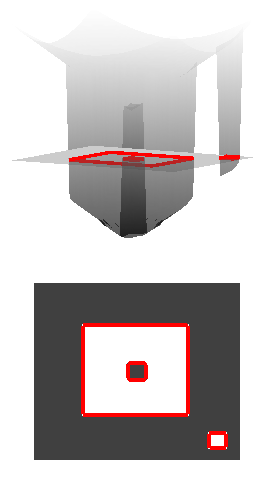
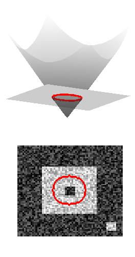
The last objective function will always select brighter region. So if the initial contour is placed in a dark area, the surface will evolve so that $\left.\phi<0\right.$ will become the bright region as shown in the figure below.

Figure 9: Wrong initialisation in region based segmentation

(a) Initial contour in dark area	(b) Intermediate step	(c) Final contour

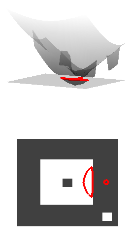
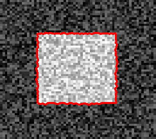
The last objective function is robust to noise as long as the noise does not change the homogeneity of each region: bright regions with noise will still remain bright, and dark regions with noise will still remain dark. The example below shows the last image with noise.

Figure 10: Region based segmentation with noise

(a) Initial contour	(b) Intermediate step	(c) Final contour

Every point on the surface is independant from its neighboring points and can have a different motion. That is why noise creates a spiky surface. Adding tension to the surface will make each point dependant from their neighbors, and it will prevent spikes. Adding a curvature term $\left.\epsilon\kappa\right.$ to the objective function gives:

$$\begin{eqnarray*} F & = & \sum_{\phi<0} \left(I(i,j)-\mu_0\right) + \sum_{\phi>0} \left(I(i,j)-\mu_1\right) + \epsilon\kappa \end{eqnarray*}$$

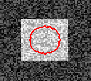
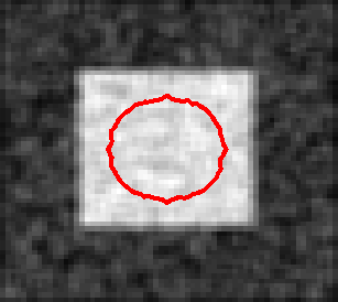
However if this term is important, sharp corners (as in a square) get lost. The example below shows the same situation as before with a little viscosity added, corners get a little bit rounded.

Figure 11: Using surface tension in a region based segmentation with noise

(a) Initial contour	(b) Intermediate step	(c) Final contour

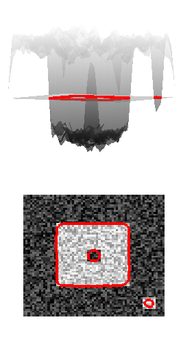
With this last result, the leaking problem has been solved. Notice also that unconnected contours, in particular inner contours are now handled.

Results

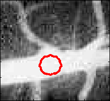
Using the previous objective function, it is now possible to segment the vessel image as shown below.

Figure 12: Vessel image using a region based objective function

(a) Initial contour	(b) Intermediate step	(c) Final contour

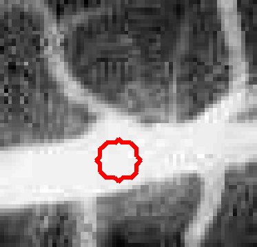
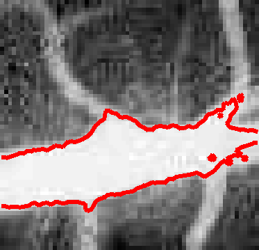
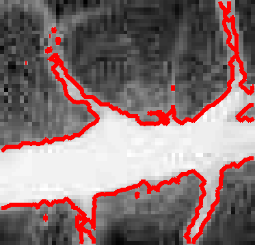
This picture shows that region based segmentation are not prune to leakage. However, the boundary may not be exactly where one think it would be. A mixture of edge based terms and region based terms in the objective function might be a good combination.