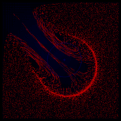
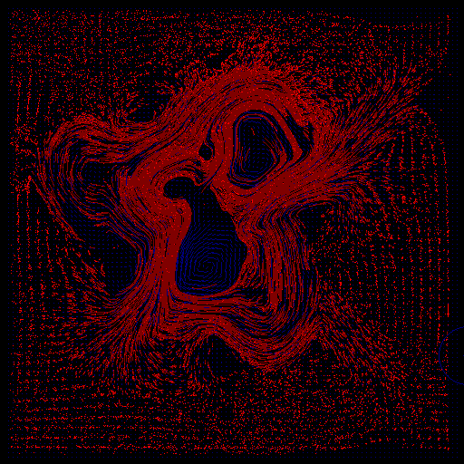
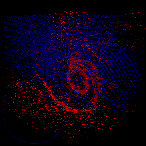
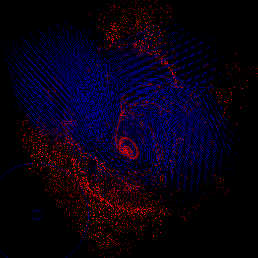
Below are screenshots of a fluid simulator, in 2D and 3D. Flow can be interactively painted onto the vector field using the mouse as a brush, effectively pushing the fluid around. In blue are the flow velocity vectors, and in red are particles moving under the effect of the vector field. The red particles are drawn with lengthened tails to indicate their direction of motion.
This started out as a test case for experimenting with vector field visualization, but later I became interested in the fluid model that generates the vector field.
The fluid model is a surprisingly simple one, based on one by Glen Murphy, downloaded from proce55ing's website and then modified. It is not meant to be accurate, but is fast, very simple to implement, and produces interesting behaviour.
The model in 2D
For each cell (x,y) in the grid, store a value p(x,y) representing "pressure" or "density" within the cell, and also store the components vx(x,y), vy(x,y) of the flow velocity through the cell. Then, for each time step of the simulation, update the cell quantities thus:
   // update p(x,y)
   for all cells (x,y) {
      px = vx(x-1,y  ) - vx(x+1,y  );
      py = vy(x  ,y-1) - vy(x  ,y+1);
      p(x,y) = (px+py)*0.5;
   }
   // update velocities
   for all cells (x,y) {
      vx(x,y) += ( p(x-1,y  ) - p(x+1,y  ) )*0.5;
      vy(x,y) += ( p(x  ,y-1) - p(x  ,y+1) )*0.5;

      if ( frictionTurnedOn ) {
         vx(x,y) *= 0.99;
         vy(x,y) *= 0.99;
      }
   }
The grid of flow velocity values vx(x,y), vy(x,y) can then be used
to accelerate particles that are carried along by the fluid.
Particle positions can be stored as floating point numbers
(i.e. they can be located anywhere within a cell; not just
at a cell's centre) and bilinear interpolation of the
vx(x,y), vy(x,y) values can be used to compute the
fluid's velocity at a particle's current position.
This interpolated fluid velocity is then used to update
the particle's velocity and position.
(Update: October 2004) After implementing the above algorithm, I learned more about vector calculus, difference equations, and numerical simulation of physical systems, and developed a better understanding of the fluid model above. It became apparent that the p field in the algorithm actually stores the (negative) divergence of the velocity field, or the net flow into each cell. Furthermore, the p field evolves according to the Heat Equation (a.k.a. Diffusion Equation), and the velocity field evolves by having the gradient of p subtracted from it at each time step. The effect of this is that the velocity field has some of its divergence removed (or diffused, actually) at each time step, and tends toward a divergence-free steady state after many time steps. A divergence-free flow is desirable, because it corresponds to the incompressibility of fluids like water. Also, in removing divergence from the velocity field, the algorithm introduces vorticity (or curl), which makes the fluid look more interesting.
Finally, the algorithm given above, although simpler and faster than Glen Murphy's original algorithm, turns out to not be the best way to simplify Murphy's. The choice of neighbours is such that we have effectively 4 independant, interlaced grids running separate simulations.